Plane wave DFG
Simulation of DFG for plane waves.
Contents
Initialize
close all;                      % Close all figures
clear all;                      % Clear all variabels
clc;                            % Clear command window
tic
Parameters
Tolerance.Abs = 1e-4;                   % Absolute tolerence
Tolerance.Rel = 1e-5;                   % Relative tolerence
Area          = pi*(40e-6)^2;
Signal.P0     = 1e6*Area;                  % Signal peak power
Idler.P0      = Signal.P0;            % Idler peak power
Pump.P0       = linspace(0.1,60,100).*1e3;  % Pump peak power
zsteps        = 5000;                   % Number of z-steps
zlength       = 60e-3;                  %Length of nonlinear crystal in [m]
plotindex     = 7;                      % Pump.P0(n) to plot in fig 3+4
QPM           = 1;                      % Use QPM or effective QPM
QPMtype       = 'eff';                  % Type of QPM: domain og eff.
Allocate memory
Signal.P    = zeros(size(Pump.P0,2),zsteps);
Idler.P     = zeros(size(Pump.P0,2),zsteps);
Pump.P      = zeros(size(Pump.P0,2),zsteps);
Total.P     = zeros(size(Pump.P0,2),zsteps);
Signal.N    = zeros(size(Pump.P0,2),zsteps);
Idler.N     = zeros(size(Pump.P0,2),zsteps);
Pump.N      = zeros(size(Pump.P0,2),zsteps);
Total.N     = zeros(size(Pump.P0,2),zsteps);
Run simulation
progressbar; % Initialize processbar

for nn=1:size(Pump.P0,2)

    % Run a 'ScalarDFG' simulation
    [z, output1, output2, output3, output4, output5, output6, output7, ...
        output8] = ScalarDFG(Tolerance.Abs, Tolerance.Rel, Signal.P0, ...
        Idler.P0, Pump.P0(nn),zsteps,zlength,QPM,QPMtype);

    % Save the calculated powers for signal and pump.
    Signal.P(nn,:)  = output1;
    Idler.P(nn,:)   = output2;
    Pump.P(nn,:)    = output3;
    Total.P(nn,:)   = output4;
    Signal.N(nn,:)  = output5;
    Idler.N(nn,:)   = output6;
    Pump.N(nn,:)    = output7;
    Total.N(nn,:)   = output8;

    % Update processbar
    progressbar( nn/size(Pump.P0,2) );

end
toc
Elapsed time is 23.956542 seconds.
Find efficiency and ignore the multiple depletion cycles
Efficiency.values = Signal.P(:,:) ./repmat(Pump.P(:,1),1,size(Signal.P,2));
Efficiency.values( floor(size(Efficiency.values,1)/2):end ...
    ,floor(size(Efficiency.values,2)*2/3):end) ...
    = 0;
[Efficiency.max.value, Efficiency.max.location] = max(Efficiency.values,[],2);
%test = sub2ind(size(Efficiency.values),1:size(Signal.P,1),transpose(Efficiency.max.location));
%Efficiency.max.plot = Efficiency.values(test);
Save workspace
%save(['Workspace-PowerPlaneWave',datestr(now, 'yyyy-mm-dd-HH-MM-SS')]);
Plots
FontSize = 18;

% waterfall plots of the pump at the different pump powers
    figure(1)
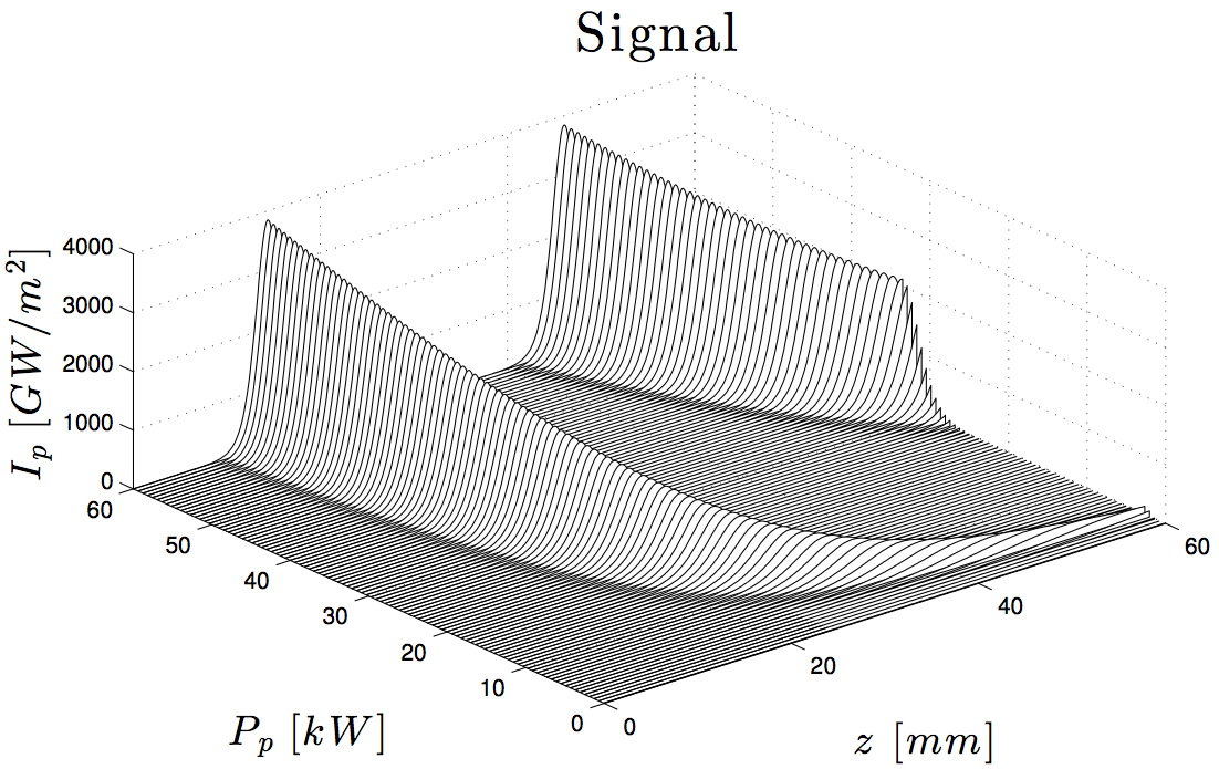
    w1 = waterfall(z(1:10:zsteps), Pump.P0.*1e-3, Signal.P(:,1:10:zsteps)./Area .*1e-9 );
    title('Signal','Interpreter','latex','FontSize',FontSize+6);
    xlabel('$z~[mm]$','Interpreter','latex','FontSize',FontSize);
    ylabel('$P_p~[kW]$','Interpreter','latex','FontSize',FontSize);
    zlabel('$I_p~[GW/m^2]$','Interpreter','latex','FontSize',FontSize);
    set(w1,'edgecolor','k');
    view([-40 50]);
    set(gca, 'Units', 'normalized','Position', [0.13 0.22 0.8 0.65]);
    set(gca, 'Color', 'none'); % Sets axes background
    export_fig PlaneWavePropagationSignal -pdf -transparent;

% waterfall plots of the signal at the different pump powers
    figure(2)
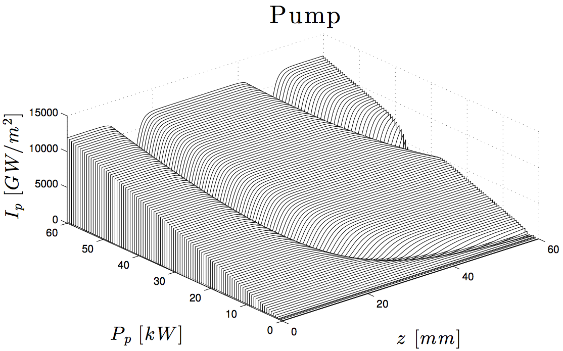
    w2 = waterfall(z(1:10:zsteps), Pump.P0.*1e-3, Pump.P(:,1:10:zsteps)./Area .*1e-9);
    title('Pump','Interpreter','latex','FontSize',FontSize+6);
    xlabel('$z~[mm]$','Interpreter','latex','FontSize',FontSize);
    ylabel('$P_p~[kW]$','Interpreter','latex','FontSize',FontSize);
    zlabel('$I_p~[GW/m^2]$','Interpreter','latex','FontSize',FontSize);
    set(w2,'edgecolor','k');
    view([-40 50]);
    set(gca, 'Units', 'normalized','Position', [0.13 0.22 0.8 0.65]);
    set(gca, 'Color', 'none'); % Sets axes background
    export_fig PlaneWavePropagationPump -pdf -transparent;

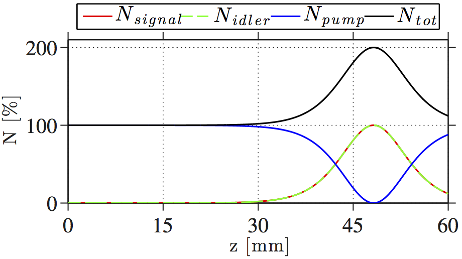
% Plots the number of photons
    figure(3)
    h3 = plot( ...
        z,Signal.N(plotindex,:)./Total.N(plotindex,1).*100,'-r', ...
        z,Idler.N(plotindex,:)./Total.N(plotindex,1).*100,'--g', ...
        z,Pump.N(plotindex,:)./Total.N(plotindex,1).*100,'-b', ...
        z,( Signal.N(plotindex,:) + Idler.N(plotindex,:) ...
        + Pump.N(plotindex,:) )./Total.N(plotindex,1).*100,'-k');
    set(h3,'LineWidth',1.5);
    l3 = legend('$N_{signal}$','$N_{idler}$','$N_{pump}$','$N_{tot}$', ...
        'Orientation','horizontal','Location','NorthOutside');
    set(l3,'Interpreter','latex')
    axis([z(1) z(end) 0 210]);
    PlotSetAxisLabels('z [mm]','N [\%]',18);
    PlotSetFigureDimensions(1,5,16,10,0,0,0,0);
    PlotSetAxisProperties(5,3,20);
    set(gca, 'Units', 'normalized','Position', [0.15 0.22 0.8 0.55]);
    set(gca, 'Color', 'none'); % Sets axes background
    export_fig PlaneWavePropagationPhoton -pdf -transparent;

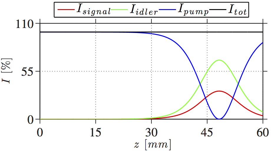
% Plots the relative power
    figure(4)
    h4 = plot( ...
        z,Signal.P(plotindex,:)./Total.P(plotindex,1).*100,'-r', ...
        z,Idler.P(plotindex,:)./Total.P(plotindex,1).*100,'-g', ...
        z,Pump.P(plotindex,:)./Total.P(plotindex,1).*100,'-b', ...
        z,( Signal.P(plotindex,:) + Idler.P(plotindex,:) ...
        + Pump.P(plotindex,:) )./Total.P(plotindex,1).*100,'-k');
    set(h4,'LineWidth',1.5);
    l4 = legend('$I_{signal}$','$I_{idler}$','$I_{pump}$','$I_{tot}$', ...
        'Orientation','horizontal','Location','NorthOutside');
    set(l4,'Interpreter','latex')
    axis([z(1) z(end) 0 110]);
    PlotSetAxisLabels('$z~[mm]$','$I~[\%]$',18);
    PlotSetFigureDimensions(1+16,5,16,10,0,0,0,0);
    PlotSetAxisProperties(5,3,20);
    set(gca, 'Units', 'normalized','Position', [0.15 0.22 0.8 0.55]);
    set(gca, 'Color', 'none'); % Sets axes background
    export_fig PlaneWavePropagationPowerRelative -pdf -transparent;

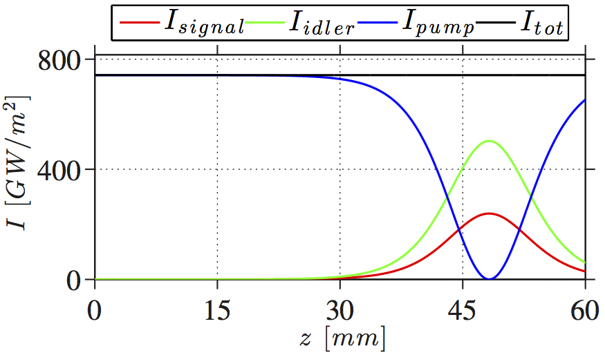
% Plots the relative power
    figure(5)
    h5 = plot( ...
        z,Signal.P(plotindex,:)./Area .*1e-9,'-r', ...
        z,Idler.P(plotindex,:)./Area .*1e-9,'-g', ...
        z,Pump.P(plotindex,:)./Area .*1e-9,'-b', ...
        z,( Signal.P(plotindex,:) + Idler.P(plotindex,:) ...
        + Pump.P(plotindex,:) )./Area .*1e-9,'-k');
    set(h5,'LineWidth',1.5);
    l5 = legend('$I_{signal}$','$I_{idler}$','$I_{pump}$','$I_{tot}$', ...
        'Orientation','horizontal','Location','NorthOutside');
    set(l5,'Interpreter','latex')
    axis([z(1) z(end) 0 1.1*max(Pump.P(plotindex,:)./Area .*1e-9)]);
    PlotSetAxisLabels('$z~[mm]$','$I~[GW/m^2]$',18);
    PlotSetFigureDimensions(1+2*16,5,16,10,0,0,0,0);
    PlotSetAxisProperties(5,3,20);
    set(gca, 'Units', 'normalized','Position', [0.2 0.22 0.75 0.55]);
    set(gca, 'Color', 'none'); % Sets axes background
    export_fig PlaneWavePropagationIrradiance -pdf -transparent;
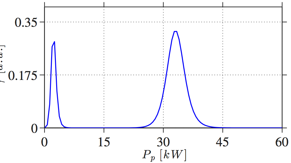
Plots the efficiency
    figure(6)
    h6 = plot( ...
        Pump.P0.*1e-3, Signal.P(:,end) ./ Pump.P(:,1));
    set(h6,'LineWidth',1.5);
    %axis([Pump.P081)*1e-3 Pump.P0(end)*1e-3 0 0.5]);
    PlotSetAxisLabels('$P_p~[kW]$','$\gamma~[a.u.]$',18);
    PlotSetFigureDimensions(1+16,5,16,10,0,0,0,0);
    PlotSetAxisProperties(5,3,20);
    set(gca, 'Units', 'normalized','Position', [0.15 0.22 0.8 0.65]);
    set(gca, 'Color', 'none'); % Sets axes background
    export_fig PlaneWaveEfficiency -pdf -transparent;

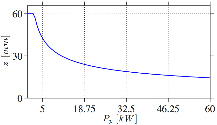
% Plots the max efficiency location
    figure(7)
    h7 = plot(Pump.P0.*1e-3, z(Efficiency.max.location));
    set(h7,'LineWidth',1.5);
    axis([Pump.P0(1)*1e-3 Pump.P0(end)*1e-3 0 1.1*max(z(Efficiency.max.location))]);
    PlotSetAxisLabels('$P_p~[kW]$','$z~[mm]$',18);
    PlotSetFigureDimensions(1+16,5,16,10,0,0,0,0);
    PlotSetAxisProperties(5,3,20);
    set(gca, 'Units', 'normalized','Position', [0.15 0.22 0.8 0.65]);
    set(gca, 'Color', 'none'); % Sets axes background
    export_fig PlaneWaveEfficiencyLocation -pdf -transparent;